Subject: NSPICE Documentation
Revision: 0.1
Date: Jan 17, 1998
Update: May 3, 1998, added screenshot NSPICEAC
Update: June 27, 1998, added archive for NSPICEAC (executable NT version)
Author: Marcel Hendrix
NSPICE, a Forth Package to Simulate Electronic Circuits
Demo
Get NSPICEAC here (nspiceac.zip 280K).
NSPICEAC is a version of NSPICE only fit for AC analysis of (simple) circuits. It demonstrates
the main features of NSPICE, among them production-quality graphics and printing. All of Forth's
power can be used in entering circuit descriptions.
Introduction
NSPICE is Not SPICE.
NSPICE is to SPICE what Forth is to C. That is, NSPICE is a personalized tool to explore a limited area of the circuit simulation field: off-line switched-mode power supply design for gas-discharge lamps. (If your interests lie elsewhere, read on).
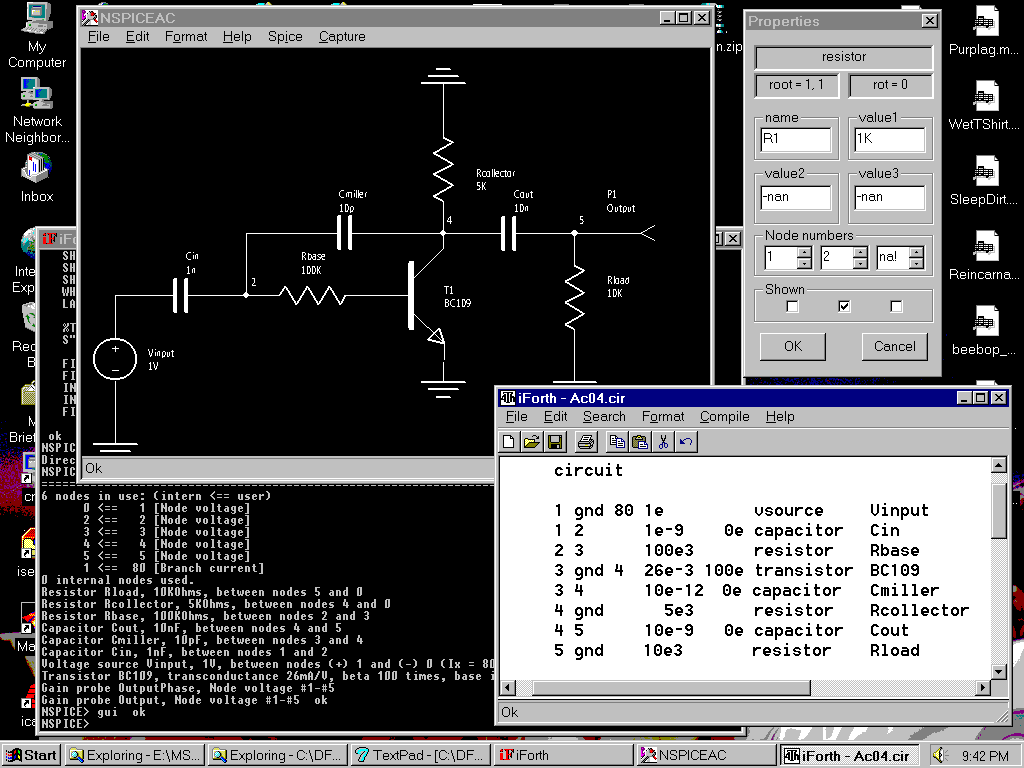
The picture below shows the typical screen layout for NSPICEAC, a variant of NSPICE designed to draw schematics and calculate AC responses. The general NSPICE is designed for TRAN calculations, but its GUI is not ready yet.
(Screenshot created with nspiceac.frt, iForth NT vsn 2.0)
 Power supply design for gas-discharge lamps is a notoriously difficult area because of the very wide range of time constants involved (mains: 20ms, rectifier-smoother: 200ms, switches 10us - 200ns, lamp 30ms - 10min).
The idea is that we can gain simulation speed by trading in generality for simplicity.
Speed is enormously important for the considered applications, as is uniform convergence.
A breakthrough is needed to enable Monte Carlo or DOE (Design Of Experiments) techniques to be applied in this area.
NSPICE doesn't use variable timesteps. The assumption (to be verified) is that these slow down switching circuits:
- there are so many corrections that the positive (speed) effect is lost
- the maximum stepsize is 1/Tswitch no matter how much cleverness is applied (actually, this is not true)
However, with fixed timesteps it is necessary to synchronize switch transitions with timesteps, to prevent excessive error as described in, e.g., "Behavior-Mode Simulation of Power Electronic Circuits", H. Jin, IEEE Transactions on Power Electronics, Vol 12, no 3, May 1997. There is a problem when the current through a switch reverses. This is a process that by definition can't be synchronized. It is obvious that in essence this is equivalent to the sampling problem in digital filters with feedback.
The problem can be reduced by reducing the timestep, but smarter, i.e less costly, algorithms might be possible. Note that resonant circuits normally don't have this problem (all discontinuities in voltages and currents appear at the switching instants), but DC-DC converters with a discontinuous mode cycle-part do suffer (as do power-feedback circuits).
The most popular remedy found in literature is interpolating all state variables back to the point where a current zero-crossing appears and restart from that point in time. This effectively "pretends" that the next timestep appears at the zero-crossing exactly, and prevents accumulating non-linear error at the cost of a small discontinuity on the time-axis. I have implemented this in the current release of NSPICE, but the effect is (disappointingly) minor.
Switch Modeling
NSPICE uses modified nodal analysis and thus needs constant, time-independent system matrices. Simulating power electronic circuits is made possible by use of the switching-function concept (Jin).
The use of switching functions transforms switched networks into a set of dependent sources (typically 2 sources per switch). The source control voltage is a function of the original switch gate turn-on/off signal. For the basic DC-DC converters the switching functions are trivial and could be made available as standard building blocks.
There are pros and cons to the switching-function concept.
Pro:
- Fast, doesn't compute the fast device level switch behavior that is mostly irrelevant for system design
- Prevents the famous problem that throwing one switch in a network generally leads to a barrage of possibly invalid intermediate states ("time must stop" while we iterate, saving and restoring states, to find the next valid state) (See: D. Bedrosian and J. Vlach, "Time-domain Analysis of Networks with Internally Controlled Switches", IEEE Trans. Circuits Syst. I, Vol 39, no 3. 1992, pp 199-212)
- The average model can be automatically derived from the switching-function description (Jin poses this as obvious)
Con:
- Switch current and voltage can get lost when the switching function is complex
- When overlap and dead-time is introduced the concept becomes difficult to use
- discontinuous mode needs a three-valued switching function
Integration Methods
H.W. Buurman, 'From Circuit to Signal; development of a piecewise linear simulator' (ETU's PLATO simulator) shows the following convergent (error->0 if h->0) and A-stable (resistant to stiff problems) integration methods (error = h^(1+order)):
- Backward Euler, order 1, u[i+1] = u[i] + h*du/dt[i+1]
- Trapezoidal, order 2, u[i+1] = u[i] + h*(du/dt[i+1]+du/dt[i])/2
- BDF (Gear), order 2, u[i+1] = 4*u[i]/3 + u[i-1]/3 + 2h*du/dt[i+1]/3
- ACF (two-step A-contractive), order 2, u[i+1] = 4*u[i]/5 + u[i-1]/5 + 2h*(5*du/dt[i+1] + 2*du/dt[i] + 2*du/dt[i-1])/15
 The dissertation also explains that "exponential integration" is not as good an idea as it may seem ("Fast Computer-Aided Simulation of Switching Power Regulators Based on Progressive Analysis of the Switches' State", Henry Shu-hung Chung and Adrian Ioinovici in ??)
On the basis of this analysis Trapezoidal Integration should be the best choice (fastest). The disadvantage of the trapezium rule is that a DC-analysis is needed before the start of a transient analysis (both Vprev and Iprev of L's and C's must be known).
Stiff ODE's
The enormous difference in fundamental timeconstants of a typical off-line converter, see above, leads to a set of "stiff" ordinary differential equations (ODE).
Stiffness is the effect that inaccurate solving of, in principle, uninteresting HF-solutions of an ODE leads to low-frequency results that are completely wrong.
The idea here is to physically separate the ODEs in fast and slow parts. This is in practice quite natural because they are generated in distinct parts of the converter anyway. A general and elegant solving method would be to simulate the circuit parts in communicating parallel processes or threads.
For a 100 kHz halfbridge on a 50 Hz mains, the tank equations are periodically solved 2,000 times per mains period (typically using 100 steps per HF-cycle).
This is clearly excessive.
Intuitively (sampling theorem) one would expect that a minimum of 100 full evaluations per second (2 per mains period) suffice.
This is not realistic given the current SOA (1997).
But even 100 evaluations per mains cycle will reduce computation time by a factor of 20.
The idea is to simulate the "fast part" accurately with a small step, over its Fast Cyclical Interval FCI (i.e. one HF switching period).
For this FCI the average voltage and current applied to the "slow part" can be computed.
The computation advances by
- assuming slow source values (these are DC input sources for the fast part)
- computing FCI with timestep Thf
- computing the slow sources (averaging over FCI at the ports to the slow part) and the new source values for the HF part
- computing the next Tlf step of the slow part
- continue at 1 (*skipping* Tlf seconds)
The method will work best when Tlf is an integer multiple of FCI.
This is no limitation.
At step 2. the new HF source values will cause the impulse response of the HF part to be triggered.
This is potentially a lowly damped oscillation.
We can simply compute n FCI cycles, where n > 1, and only keep the last step.
This can be automated, however, when n > Tlf/FCI there is no gain in our new method.
Methods exist to compute the PSS in a single step, we may use them in the future.
Finally, some (current-mode) circuits do not have a constant FCI, it varies during the simulation.
This is not important for the method explained above.
The implementation in NSPICE is such that this is not a problem for the simulator anymore.
Note that the described method is related to state-space averaged modeling.
However, we don't require the user to derive switch and converter models analytically, the simulator does this numerically, on-the-fly.
Moreover, this technique doesn't require low ripple, a periodical steady state is all that is required.
Also, contrary to SSA we get HF detail and LF response at the same time while current-mode control and discontinuous mode aren't problematic (when the proper switch models are being used).
Errors
Above I stated: `The idea is to simulate the "fast part" accurately with a small step'.
Actually, this is quite a problem because errors in the FCI get at least multiplied by RATE-MAX (to first order approximation).
This means that for a global error < 0.1%, assuming RATE-MAX <= 1000, we need a basic accuracy of 1e-6 over the FCI.
Because we use trapezoidal integration (error proportional to h^3) we need h on the order FCI/1e2, assuming 100% error for h = FCI.
(In practice it is easy to find signals that have much larger errors--a diode switching off at the start of the FCI, etc.).
For a basic accuracy of 1% and well behave signals we still need on the order of 50 steps on the FCI.
Therefore, for future releases, it might be needed to complicate matters and go back to variable, quality-controlled, timesteps.
Not all bad, as this automatically solves the "unsynchronized event problem" (diodes turning on or off between timesteps).
Hopefully the increased overhead per step is compensated by the fact that larger steps can be taken.
The fact that it is very difficult to beat SPICE for non-stiff SMPS circuits is encouraging here.
A "problem" with variable timestep, aka non-constant system matrix, is that ALL states must be stored in the system matrix.
Implementation of e.g. a flip-flop or averager using local variables is out of the question.
Extension A:
We may have to go to variable timesteps (and thus setting up and solving a new system matrix once each timestep).
The alternative is to redo the FCI with a smaller Thf.
The results should be identical within some error bound.
If not, decrease Thf and restart the FCI computation.
This is a much less costly extension because a new system matrix must be set up and solved, only twice per FCI (not once per timestep).
Because of our definition of FCI, all FCIs are equal so the Thf is constant during the simulation once the optimal value has been found.
It is always possible to do a simulation twice and compare the results to see if it has to be redone with smaller Thf (a prudent user will do this anyway).
This is certainly more efficient than the dynamic step method for a single simulation, and it is much, much more efficient for Monte Carlo analysis.
However, there might be circuits for which the needed Thf is so small that the variable time step method would have been more efficient after all.
This can only be found experimentally.
Unless we have a "special" circuit at hand, it seems the main benefit of this extension is with naive users, or when it is considered "unprofessional" to have the user explicitly check the validity of the results.
This is not our target audience; and so we won't implement this extension A (not now anyway :).
Extension B:
Check if the state variables changed "negligeably" after computing an FCI.
(This is stricter, and, amazingly, easier to compute, than checking if they're independent of Thf).
If they don't, compute another FCI until they do, else skip to the next LF point.
This checks that the "FCI" is indeed cyclical, i.e that there are no relatively "fast" dynamics.
This doesn't guarantee correct results when the Tlf is chosen too large (Ext. C).
It looks to me that this strategy prevents accumulating large errors when making a Tlf step excites the impulse response of the HF part.
This seems like a very useful addition (a formal PSS solver would be better).
Extension C:
Check if the averaged state variables depend on the value of Tlf. If they do, decrease Tlf and restart.
See also Extension A: this isn't useful when we can (and should) redo the complete simulation.
The alternative is to check if the averaged state variables change "too much" and issue a WARNING when true (this is too strict because it will warn for perfectly valid transients as well).
Beacuse of the implementation, decreasing Tlf means that the system matrix must be recomputed and solved again.
Therefore, once Extension C is done there is no reason to not implement Extension A (alternative part).
Implementation
In practice it is not necessary to laboriously calculate average values at the FAST <==> SLOW ports.
The effect of Tstep on the fast and slow circuit matrices is concentrated in the C, L elements: h/C and h/L terms.
A larger Tstep is clearly equivalent with smaller C and L values.
Thus it is sufficient to use Tlf/Thf times down-scaled L and C values in the slow part, computing both parts at once with the same (small) Thf. It remains to detect the boundaries of the HF PSS (trivial in a fixed frequency circuit) and to discontinuously advance time to the next (Tlf) point.
16 Nov 1997: For the first try we disregarded the HF-PSS problem (assume high damping).
First we solve the equations over the [given, required] FCI using Thf.
The SLOW circuit parts are identified and the C, L values scaled down by RATE=Tlf/Thf. RATE is entered by the user, Tlf is an internal parameter.
The main loop advances ntime by Tlf when ntime = k*Tlf+FCI.
There's of course a (user interface) problem when plotting the results (plot the FCI-averaged values of the state variables when k*Tlf+FCI < ntime < (k+1)*Tlf)
Thoughts & Ideas
At the time of writing, Jan 17, 1998, I have worked with NSPICETR intensively over a period of 3 months.
The simulation speed is very high: 33 - 100 times faster than SPICE on realistic circuits.
Personally I like the input method better than SPICE's.
In the future I will want a schematic drawing of the netlist, but for small projects it is no problem yet.
The flexibility of NSPICE's ASCII input for procedures, macros and simulation specification has no match in SPICE, I doubt if I'll ever consider adding schematic entry.
The NSPICE post-processor, although spartan, does most of what I need and allows high quality display, clipboarding and printing. For big jobs INTUSCOPE is used as an additional post-processor, working as a background task in a separate window.
The extensions listed above don't seem to matter much, for the practical circuits tried up to now.
The visual feedback from the simulator immediately points out wrongly assigned FCI or RATE constants, and the user can almost instantly correct this.
Specifically, I do not believe that having perfect state-event signalling/handling, or higher-order multistep integration (with non-constant state matrix) will bring much for SMPS simulation (simulating switched capacitor filters would be an entirely different kettle of fish).
NSPICE speed can be increased for special problems.
I now keep Tlf constant, but could design some sort of "quality-controlled" Tlf stepper.
The system matrix must be recomputed if Tlf changes, on the other hand the positive effect is high when analyzing, e.g., the impulse response of a SMPS.
The VRES component implementation has already shown how to handle a "database" of system matrices, so this might be an easy job.
NSPICE overview
Circuit Segmentation
CIRCUIT -- required at top of file. No END needed.
[pss] FAST( )FAST -- Pseudo Steady-State interval of fast process
[rate] SLOW( )SLOW -- # of PSSs the slow process skips
Basic Components
RESISTOR
CAPACITOR
INDUCTOR
JSOURCE
VSOURCE
USOURCE
UJSOURCE
TRANSFORMER
V->V
Advanced Models
DIODE-SW
HB-SWITCH
RESO-SW
R-SWITCH
DIODE
DIODEX
VRES
Macro Models
PWM-FIXED
PWM-FIXED+T
PWM
COMPARATOR
FLIP-FLOP
DRIVER
ABS-SINE
ABS-COSINE
FULL-SINE
SQUARE-WAVE
NEW-FCI -- helps with current-mode control, FM and such
Displaying Results
GPROBE
-GPROBE
GDPROBE
GXYPROBE
TV
-TV
DTV
PTV
XYTV
PROBE
-PROBE
DPROBE
W:LBOTTOM
W:RBOTTOM
W:BOTTOM
W:L1
W:R1
W:XX
(more) ... plotwindows
Specifying the simulation parameters
[Tbegin] [Tend] [Tstep] TRANSIENT-PLOT
[Tbegin] [Tend] [Tstep] TRAN-PLOT-FAST
[Tbegin] [Tend] [Tstep] TRANSIENT-TABLE
REFRESH
REPAINT -- refresh display (needed when simulator is inactive)
<#ms> TO FRAMERATE
TRUE | FALSE TO ERASE?
TRUE | FALSE TO RMS?
Postprocessing
WHITE-PAGE
BLACK-PAGE
WHEN ( "name" -- bool )
LABELS" fname"
SHOW1 CLIP1 PRINT1 ( CLIPnnn PRINTnn only available for Windows )
SHOW2 CLIP2 PRINT2 SHOW2x2 CLIP2x2 PRINT2x2
SHOW3 CLIP3 PRINT3 SHOW3x2 CLIP3x2 PRINT3x2
SHOW5 CLIP5 PRINT5 SHOW5x2 CLIP5x2 PRINT5x2 (>-versions of all these)
.INFO
.REPORT
.STATIC
.SOLUTION
.DUMPS" filename"
%TOL
%TOLG
%TOLG-LOW
%TOLG-HIGH -- tolerances Monte-Carlo analysis
S" include fname" #cases #bins CASES -- perform Monte-Carlo run
free counter

 Power supply design for gas-discharge lamps is a notoriously difficult area because of the very wide range of time constants involved (mains: 20ms, rectifier-smoother: 200ms, switches 10us - 200ns, lamp 30ms - 10min).
The idea is that we can gain simulation speed by trading in generality for simplicity.
Speed is enormously important for the considered applications, as is uniform convergence.
A breakthrough is needed to enable Monte Carlo or DOE (Design Of Experiments) techniques to be applied in this area.
 The dissertation also explains that "exponential integration" is not as good an idea as it may seem ("Fast Computer-Aided Simulation of Switching Power Regulators Based on Progressive Analysis of the Switches' State", Henry Shu-hung Chung and Adrian Ioinovici in ??)